Given a simple motion path, we can derive the necessary torques at each joint in a robotic arm in order for the end-effector to trace the desired path. (Torque is a stand-in for current to a motor, albeit leaving out the stall characteristics)

Assumptions: Assume friction/drag are negligible, the masses of the linkages are known and evenly distributed, and the joints represent perfect motors (no torque curves).

Joint-Frame Translation Matrices

Forward Kinematics

Forward kinematics is used to take the robot parameters (angles) and produce a position and orientation of the end-effector. In our case, we simplify the equation a bit since we consider the end effector as a point instead of an end-effector with complex geometry.

To go from the fixed frame \(F\) at the origin to the final frame \(M_3\) which represents the end-effector, we want to calculate $$F \rightarrow M_1 \rightarrow M_2 \rightarrow M_3$$

Thus, we want to solve for the following homogeneous transforms: $$\begin{align*} H &= F \rightarrow M_1 \rightarrow M_2 \rightarrow M_3\\ &= (F \rightarrow M_1)(M_1 \rightarrow M_2)(M_2 \rightarrow M_3)\\ &= H_1H_2H_3 \end{align*}$$

Thus, \(H = F \rightarrow M_3\).

In the top left of the \(3 \times 3\) homogeneous transform matrix, we place the \(2 \times 2\) rotation matrix and in the last column, we include the displacement (within that frame): $$\begin{align*} \begin{bmatrix} \cos \theta & -\sin \theta & disp_x\\ \sin \theta & \cos \theta &disp_y\\ 0 & 0 & 1 \end{bmatrix} \end{align*}$$

Forward Kinematics Example

Let us calculate the forward kinematics for the example shown:

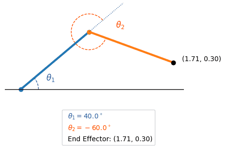
$$\begin{align*} H &= H_1H_2H_3\\ &= \begin{bmatrix} \cos (40 ^{\circ}) & -\sin (40 ^{\circ}) & 0\\ \sin (40 ^{\circ}) & \cos (40 ^{\circ}) &0\\ 0 & 0 & 1 \end{bmatrix} \begin{bmatrix} \cos (-60 ^{\circ}) & -\sin (-60 ^{\circ}) & 1\\ \sin (-60 ^{\circ}) & \cos (-60 ^{\circ}) &0\\ 0 & 0 & 1 \end{bmatrix} \begin{bmatrix} 1 & 0 & 1\\ 0 & 1 &0\\ 0 & 0 & 1 \end{bmatrix}\\ % &= \begin{bmatrix} 0.7660 & -0.6428 & 0\\ 0.6428 & 0.7660 &0\\ 0 & 0 & 1 \end{bmatrix} \begin{bmatrix} 0.5 & 0.8660 & 1\\ -0.8660 & 0.5 &0\\ 0 & 0 & 1 \end{bmatrix} \begin{bmatrix} 1 & 0 & 1\\ 0 & 1 &0\\ 0 & 0 & 1 \end{bmatrix}\\ % &= \begin{bmatrix} 0.9397 & 0.342 & 1.7057\\ -0.342 & 0.9397 & 0.3008\\ 0 & 0 & 1 \end{bmatrix} \end{align*} $$

The top left \( 2 \times 2 \) matrix is the rotation of the end-effector:

$$\begin{align*} \begin{bmatrix} 0.9397 & 0.342 & 1.7057\\ -0.342 & 0.9397 & 0.3008\\ 0 & 0 & 1 \end{bmatrix} &= \begin{bmatrix} \cos \theta & -\sin \theta & disp_x\\ \sin \theta & \cos \theta &disp_y\\ 0 & 0 & 1 \end{bmatrix} \end{align*}$$

Since \( \cos \theta = 0.9397 \) and \( \sin \theta = -0.342 \), then:

$$\begin{align*} \theta &= \tan^{-1} \bigg(\frac{-0.342}{0.9397}\bigg)\\ &= \tan^{-1} (-0.364)\\ &\approx -20 ^{\circ} \end{align*}$$

The last column is the total displacement from the origin frame to the end-effector and thus gives the end-effector’s position and rotation is:$$(1.71, 0.30, -20 ^{\circ})$$

Inverse Kinematics

Calculating inverse kinematics is the process of calculating the intermediate homogeneous transform matrices given \(H\):

$$\begin{align*} H &= H_1H_2H_3 \\ &= \begin{bmatrix} \cos (\theta_1) & -\sin (\theta_1) & 0\\[3pt] \sin (\theta_1) & \cos (\theta_1) & 0\\[3pt] 0 & 0 & 1 \end{bmatrix} \begin{bmatrix} \cos (\theta_2) & -\sin (\theta_2) & 1\\[3pt] \sin (\theta_2) & \cos (\theta_2) & 0\\[3pt] 0 & 0 & 1 \end{bmatrix} \begin{bmatrix} 1 & 0 & 1 \\[3pt] 0 & 1 & 0\\[3pt] 0 & 0 & 1 \end{bmatrix}\\ &= \begin{bmatrix} \cos (\theta_1) & -\sin (\theta_1) & 0\\[3pt] \sin (\theta_1) & \cos (\theta_1) & 0\\[3pt] 0 & 0 & 1 \end{bmatrix} \begin{bmatrix} \cos (\theta_2) & -\sin (\theta_2) & \cos (\theta_2) + 1\\[3pt] \sin (\theta_2) & \cos (\theta_2) & \sin (\theta_2)\\[3pt] 0 & 0 & 1 \end{bmatrix}\\ &= \begin{bmatrix} \cos\theta_1\cos\theta_2 -\sin\theta_1\sin\theta_2 & -\bigl(\cos\theta_1\sin\theta_2 + \sin\theta_1\cos\theta_2\bigr) & \cos\theta_1(\cos\theta_2+1)\;-\;\sin\theta_1\sin\theta_2 \\[3pt] \sin\theta_1\cos\theta_2 +\cos\theta_1\sin\theta_2 & \cos\theta_1\cos\theta_2 – \sin\theta_1\sin\theta_2 & \sin\theta_1(\cos\theta_2+1)\;+\;\cos\theta_1\sin\theta_2 \\[3pt] 0 & 0 & 1 \end{bmatrix}\\ &= \begin{bmatrix} \cos(\theta_1+\theta_2) & -\sin(\theta_1+\theta_2) & \cos(\theta_1+\theta_2)+\cos\theta_1\\[3pt] \sin(\theta_1+\theta_2) & \cos(\theta_1+\theta_2) & \sin(\theta_1+\theta_2)+\sin\theta_1\\[3pt] 0 & 0 & 1 \end{bmatrix} \end{align*}$$

Let our desired end-effector pose be represented as the matrix:

$$\begin{align*} H &= \begin{bmatrix} \cos (\theta_{end}) & -\sin (\theta_{end}) & x_{end}\\ \sin (\theta_{end}) & \cos (\theta_{end}) &y_{end}\\ 0 & 0 & 1 \end{bmatrix} \end{align*}$$

We can then create a system of equations and solve for the angles of the robotic arm. However, we’re going to simplify our pose by disregarding orientation of end-effector and simply solving for the displacement. Thus yielding the following system:$$\begin{align*} x_{end} &= \cos (\theta_1) + \cos(\theta_1 + \theta_2),\\ y_{end} &= \sin(\theta_1) + \sin(\theta_1 + \theta_2) \end{align*}$$

First, to simplify further algebra and decouple the variables, we introduce the distance from the origin to the end-effector:

$$\begin{align*} r^2 &:= (x_{end})^2 + (y_{end})^2\\ &= (\cos (\theta_1) + \cos(\theta_1 + \theta_2))^2 + (\sin(\theta_1) + \sin(\theta_1 + \theta_2))^2\\ &= \cos^2 (\theta_1) + \cos^2(\theta_1 + \theta_2) + 2\cos (\theta_1) \cos(\theta_1 + \theta_2) \\&\ \ \ \ + \sin^2 (\theta_1) + \sin^2(\theta_1 + \theta_2) + 2\sin (\theta_1) \sin(\theta_1 + \theta_2)\\ &= \big[\cos^2 (\theta_1) + \sin^2 (\theta_1)\big] + \big[\cos^2(\theta_1 + \theta_2)+ \sin^2(\theta_1 + \theta_2)\big] \\&\ \ \ \ + 2\cos (\theta_1) \cos(\theta_1 + \theta_2) + 2\sin (\theta_1) \sin(\theta_1 + \theta_2)\\ &= 1 + 1 + 2\big[\cos (\theta_1) \cos(\theta_1 + \theta_2) + \sin (\theta_1) \sin(\theta_1 + \theta_2)\big]\\ &= 2 + 2\cos ((\theta_1 + \theta_2) – \theta_1) \text{($\cos (A-B) = \cos A \cos B + \sin A \sin B$)}\\ r^2 &= 2 + 2 \cos (\theta_2) \end{align*}$$

To solve for \( \theta_2 \), we can now do:

$$\begin{align*} r^2 &= 2 + 2 \cos (\theta_2)\\ \cos (\theta_2) &= \frac{r^2 -2}{2}\\ \theta_2 &= \pm \arccos \bigg(\frac{r^2 – 2}{2}\bigg)\\ \theta_2 &= \pm \arccos \bigg(\frac{(x_{end})^2 + (y_{end})^2 – 2}{2}\bigg) \end{align*}$$

where the \( \pm \) represents elbow up or elbow down configurations.

To solve for \( \theta_1 \), we use the sum to product formula to derive:

$$\begin{align*} x_{end} &= \cos (\theta_1) + \cos (\theta_1 + \theta_2)\\ &= 2\cdot \cos (\theta_1 + \tfrac{\theta_2}{2})\cdot\cos(\tfrac{\theta_2}{2})\\ y_{end} &= \sin (\theta_1) + \sin(\theta_1 + \theta_2)\\ &= 2\cdot \sin\big(\theta_1 + \tfrac{\theta_2}{2})\cdot \cos (\tfrac{\theta_2}{2}) \end{align*}$$

We can then form the following since the \( \cos(\tfrac{\theta_2}{2}) \) and \( 2 \) cancel:

$$\begin{align*} \tan (\theta_1 + \tfrac{\theta_2}{2}) &= \frac{y_{end}}{x_{end}}\\ \theta_1 + \tfrac{\theta_2}{2} &= \text{atan2} (y_{end}, x_{end})\\ \theta_1 &= \text{atan2} (y_{end}, x_{end}) – \tfrac{\theta_2}{2} \end{align*}$$

Inverse Kinematics Example

Recall the forward kinematics example end-effector coordinate: $$(1.71, 0.30)$$

Let us calculate the joint configurations for the end-effector to reach this coordinate (disregarding end-effector angle for simplicity):

$$\begin{align*} \theta_2 &= \pm \arccos \bigg(\frac{(x_{end})^2 + (y_{end})^2 – 2}{2}\bigg)\\ &= \pm \arccos \bigg(\frac{(1.71)^2 + (0.3)^2 – 2}{2}\bigg)\\ &= \pm \arccos (0.50705)\\ &\approx \{-59.533, 59.533\} \end{align*}$$

Let’s use the positive angle first:

$$\begin{align*} \theta_1 &= \text{atan2} (y_{end}, x_{end}) – \tfrac{\theta_2}{2}\\ &= \text{atan2} (0.3, 1.71) – \tfrac{1.03904686}{2}\\ &\approx 0.174 – 0.51952343\\ &\approx= -0.346 = -19.82 ^{\circ} \end{align*}$$

then solve using the negative angle:

$$\begin{align*} \theta_1 &= \text{atan2} (y_{end}, x_{end}) – \tfrac{\theta_2}{2}\\ &= \text{atan2} (0.3, 1.71) – \tfrac{-1.03904686}{2}\\ &\approx 0.174 + 0.51952343\\ &\approx= 0.69352343 = 39.74 ^{\circ} \end{align*}$$

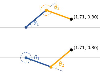
Thus, we obtained two valid configuration solutions, one that represents “elbow up” and the other for “elbow down”:

Inverse Kinematics Solvers

Putting IK to use requires us to avoid several caveats such as singularities or switching IK “branches”. For example, we can induce a singularity by traversing a shape like:

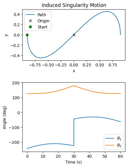
We can avoid these, if in our inverse kinematics function we incorporate a simple “angle-distance” check to our last position, allowing for circular overflow. See the Code section for our IK solver.

Inverse Dynamics

Lagrangian

At a high-level, Newtonian mechanics breaks mechanical problems down into forces while Lagrangian methods focuses on energy as its fundamental unit of measure.

The definition of the Lagrangian for a dynamic system is as follows: $$\begin{align*} L &= K – P\\ L &= \text{(kinetic energy)} – \text{(potential energy)} \end{align*}$$

Let us represent the angles, angular velocities, and angular accelerations as vector functions:

$$\begin{align*} \theta(t) = \begin{bmatrix} \theta_1\\\theta_2 \end{bmatrix}(t),\quad \dot{\theta}(t) = \begin{bmatrix} \dot{\theta_1}\\\dot{\theta_2} \end{bmatrix}(t),\quad \ddot{\theta}(t) = \begin{bmatrix} \ddot{\theta_1}\\\ddot{\theta_2} \end{bmatrix}(t) \end{align*}$$

Thus, the kinetic energy depends on the pose and the joints’ velocities while the potential energy (due to gravity) only depends on the pose. And therefore, the Lagrangian is simply a function of the pose and angles’ velocities as well:

$$\begin{align*} L(\theta, \dot{\theta}) &= K(\theta, \dot{\theta}) – P(\theta) \end{align*}$$

To solve for the Lagrangian, we start filling out the equation with known quantities.

Kinetic Energy

To solve for the kinetic energy in the system, we sum the translational and rotational energy for each of the linkage masses (assuming the joints have negligible mass).

Translational Kinetic Energy

Let us find the center of mass (COM) as a function of the angles, then take the derivative to get the velocity of each linkage in Cartesian space as a function of the angles and angles’ velocities.

Let \( (x_{i},\ y_{i}) \) represent the Cartesian location of the center of mass of the \( i \)-th linkage. Using trigonometry/geometry we find that the centers of mass are: $$\begin{align*} x_1 = \frac{l_1}{2}\cos (\theta_1), \quad y_1 = \frac{l_1}{2}\sin (\theta_1) \end{align*}$$ and $$\begin{align*} x_2 = l_1\cos (\theta_1) + \frac{l_2}{2}\cos(\theta_1 + \theta_2), \quad y_2 =l_1\sin (\theta_1) + \frac{l_2}{2}\sin(\theta_1 + \theta_2) \end{align*}$$ for links \( 1 \) and \( 2 \) respectively.

Now that we have the positions of each linkages’ center of mass as a function of the angles, we can differentiate with respect to time to get the velocities of each joint.

Since we want to differentiate a function of the form \( f(\theta, \theta_2) \) with respect to time, we use the chain rule to expand it: $$\begin{align*} \frac{d}{dt}f(\theta, \theta_2) &= \frac{\partial f}{\partial \theta_1}\dot{\theta_1} + \frac{\partial f}{\partial \theta_2}\dot{\theta_2} \end{align*}$$ Thus, the velocities of each center of mass become:

$$\begin{align*} \dot{x_1} &= -\frac{l_1}{2} \sin (\theta_1)\cdot \dot{\theta_1}\\ \dot{y_1} &=\frac{l_1}{2}\cos(\theta_1)\cdot \dot{\theta_1} \end{align*}$$

and

$$ \begin{align*} \dot{x_2} &= -l_1 \sin (\theta_1)\cdot \dot{\theta_1} – \frac{l_2}{2} \sin(\theta_1 + \theta_2)\cdot (\dot{\theta_1} + \dot{\theta_2})\\ \dot{y_2} &= l_1\cos(\theta_1)\cdot \dot{\theta_1} + \frac{l_2}{2}\cos(\theta_1 + \theta_2)\cdot (\dot{\theta_1} + \dot{\theta_2}) \end{align*}$$

Recall the equation for the kinetic energy of a moving object: $$KE = \frac{1}{2}mv^2$$

To obtain the velocity-squared component for the first link (\( v_1 \)) we use the Pythagorean Theorem:

$$\begin{align*} v_1^2 &= \dot{x_1}^2 + \dot{y_1}^2\\ &= \bigg(-\frac{l_1}{2}\sin(\theta_1)\cdot \dot{\theta_1}\bigg)^2 + \bigg(\frac{l_1}{2}\cos(\theta_1)\cdot \dot{\theta_1}\bigg)^2\\ &= \frac{{l_1}^2}{4}\big(\sin^2(\theta_1) + \cos ^2 (\theta_1)\big)\cdot\dot{\theta_1}^2\\ &= \frac{{l_1}^2}{4}\cdot\dot{\theta_1}^2 \end{align*}$$

Then, for the second link:

$$\begin{align*} v_2^2 &= \dot{x_2}^2 + \dot{y_2}^2\\ &= \bigg(-l_1 \sin (\theta_1)\cdot \dot{\theta_1} – \tfrac{l_2}{2} \sin(\theta_1 + \theta_2)\cdot (\dot{\theta_1} + \dot{\theta_2})\bigg)^2 \\ &\ \ \ \ + \bigg(l_1\cos(\theta_1)\cdot \dot{\theta_1} + \frac{l_2}{2}\cos(\theta_1 + \theta_2)\cdot (\dot{\theta_1} + \dot{\theta_2})\bigg)^2\\ &= {l_1}^2\dot{\theta_1}^2 + \tfrac{{l_2}^2}{4}\big(\dot{\theta_1} + \dot{\theta_2}\big)^2 \\ &\ \ \ \ + 2\big(-l_1\sin (\theta_1)\cdot \dot{\theta_1}\big)\cdot\big(-\tfrac{l_2}{2}\sin(\theta_1 + \theta_2)\cdot (\dot{\theta_1} + \dot{\theta_2})\big) \\ &\ \ \ \ + 2\big(l_1\cos(\theta_1)\cdot \dot{\theta_1}\big)\cdot \big(\tfrac{l_2}{2}\cos(\theta_1 + \theta_2)\cdot (\dot{\theta_1} + \dot{\theta_2})\big)\\ &= {l_1}^2\dot{\theta_1}^2 + \frac{{l_2}^2}{4}(\dot{\theta_1} + \dot{\theta_2})^2 + l_1l_2\dot{\theta_1}(\dot{\theta_1} + \dot{\theta_2})\cdot \cos (\theta_2) \end{align*}$$

Rotational Kinetic Energy

Now we need the rotational kinetic energy of each linkage. We know the rotational inertia of a uniform rod about it’s center of mass is: $$I_i = \frac{1}{12}m_i{l_i}^2$$

Recall also that the rotational energy is: $$K_{rot_i} = \tfrac{1}{2}I_i{\omega_i}^2$$

where the angular speeds are simply: \( \omega_1 = \dot{\theta_1} \) and \( \omega_2 = \dot{\theta_1} + \dot{\theta_2} \).

Therefore, the kinetic energy of the linkages is the sum of their translational and rotational energies:

$$\begin{align*} K(\theta, \dot{\theta}) &= \big[\tfrac{1}{2}m_1{v_1}^2 + \tfrac{1}{2}m_2{v_2}^2\big] + \big[\tfrac{1}{2}I_1\dot{\theta_1}^2 + \tfrac{1}{2}I_2(\dot{\theta_1} + \dot{\theta_2})^2\big] \end{align*}$$

Potential Energy

The potential energy in our system is gravitational potential energy: $$PE = mgh$$

Thus, $$\begin{align*} P(\theta) &= m_1 y_1 g + m_2 y_2 g,\quad g \approx 9.81\ m/s^2\\ &= m_1g\frac{l_1}{2}\sin(\theta_1) + m_2g(l_1\sin (\theta_1) + \frac{l_2}{2}\sin(\theta_1 + \theta_2)) \end{align*}$$

Euler-Lagrangian

The Euler-Lagrangian equation derivation is beyond the scope of this project (mainly dealing with differential equations and equations of motion). It comes from a variational principle, e.g. Hamilton’s principle of stationary action or D’Alembert’s principle of virtual work.

In our case, the generalized force conjugate to \( \theta_i \) is the torque \( \tau_i \):

$$\begin{align*} \tau_i &= \frac{d}{dt}\bigg(\frac{\partial L}{\partial \dot{\theta_i}}\bigg) – \frac{\partial L}{\partial \theta_i} \end{align*}$$

Let’s start by computing the partial derivative of the Lagrangian with respect to the velocity \( \dot{\theta_i} \). We observe that the potential energy does not depend on velocity, so we can simplify our calculations to be just: $$\frac{\partial L}{\partial \dot{\theta_i}} = \frac{\partial K}{\partial \dot{\theta_i}}$$

By utilizing the concept of a manipulator inertia matrix (or “mass matrix”), we can group/rewrite the kinetic energy into:

$$\begin{align*} K\bigg(\begin{bmatrix} \theta_1\\\theta_2 \end{bmatrix}, \begin{bmatrix} \dot{\theta_1}\\\dot{\theta_2} \end{bmatrix}\bigg) &= \tfrac{1}{2}\begin{bmatrix} \dot{\theta_1} & \dot{\theta_2} \end{bmatrix} \begin{bmatrix} M_{11} & M_{21}\\M_{12} & M_{22} \end{bmatrix}\begin{bmatrix} \dot{\theta_1}\\\dot{\theta_2} \end{bmatrix}\\ % &\text{($M_{12} = M_{21}$) due to symmetry}\\ &= \tfrac{1}{2}M_{11}\dot{\theta_1}^2 + M_{12}\dot{\theta_1}\dot{\theta_2} + \tfrac{1}{2}M_{22}\dot{\theta_2}^2 \end{align*}$$

Where the manipulator inertia matrix is defined as:

$$\begin{align*} M(\theta) &= \begin{bmatrix} I_1 + I_2 + \frac{m_1{l_1}^2}{4} + m_2({l_1}^2 + \frac{{l_2}^2}{4} + l_1l_2\cos(\theta_2)) & I_2 + m_2(\frac{{l_2}^2}{4} + \frac{l_1l_2}{2}\cos (\theta_2))\\ I_2 + m_2 (\frac{{l_2}^2}{4} + \frac{l_1l_2}{2}\cos (\theta_2)) & I_2 + \frac{m_2{l_2}^2}{4} \end{bmatrix} \end{align*}$$

Thus, explicitly we have:

$$\begin{align*} \frac{\partial K}{\partial \dot{\theta_1}} &= M_{11}\dot{\theta_1} + M_{12}(\dot{\theta_1} + \dot{\theta_2}), \quad \frac{\partial K}{\partial \dot{\theta_2}} = M_{12}\dot{\theta_1} + M_{22}(\dot{\theta_1} + \dot{\theta_2}) \end{align*}$$

or we can write simply:

$$\begin{align*} \frac{\partial K}{\partial \dot{\theta}} &= \frac{\partial L}{\partial \dot{\theta}} = M(\begin{bmatrix} \theta_1\\\theta_2 \end{bmatrix})\begin{bmatrix} \dot{\theta_1}\\\dot{\theta_2} \end{bmatrix}= M(\theta)\dot{\theta} \end{align*}$$

Then, to take the derivative with respect to time, we get:

$$\begin{align*} \frac{d}{dt}\bigg( \frac{\partial L}{\partial \dot{\theta_i}}\bigg) &= M(\theta)\ddot{\theta} + C(\theta, \dot{\theta}) \dot{\theta} \end{align*}$$

where the term \( C(\theta, \dot{\theta})\cdot \dot{\theta} \) (or Coriolis–a velocity product term) satisfies the following:

$$\begin{align*} C(\theta, \dot{\theta})\cdot \dot{\theta} &= \begin{bmatrix} -m_2 l_1 \frac{l_2}{2} \sin (\theta_1) \dot{\theta_2} (\dot{\theta_1} + \dot{\theta_2})\\ m_2 l_1 \frac{l_2}{2} \sin(\theta_2) \dot{\theta_1}^2 \end{bmatrix} \end{align*}$$

Lastly, we compute the partial derivative of the Lagrangian with respect to the angles \( \frac{\partial L}{\partial \theta_i} \):

$$\begin{align*} \frac{\partial L}{\partial \theta_i} &= \frac{\partial K}{\partial \theta_i} – \frac{\partial P}{\partial \theta_i} \end{align*}$$

Since we already solved for the potential energy with:

$$\begin{align*} P &= m_1g\frac{l_1}{2}\sin(\theta_1) + m_2g(l_1\sin P(\theta_1) + \frac{l_2}{2}\sin(\theta_1 + \theta_2)) \end{align*}$$

Taking the partial derivative with respect to each angle, we obtain:

$$\begin{align*} \frac{\partial P}{\partial \theta_1} &= m_1g\frac{l_1}{2}\cos (\theta_1) + m_2g(l_1\cos (\theta_1) + \frac{l_2}{2}\cos(\theta_1 + \theta_2)),\\ \frac{\partial P}{\partial \theta_2} &= m_2g\frac{l_2}{2}\cos(\theta_1 + \theta_2) \end{align*}$$

Then, for the kinetic energy term, we also find the partial derivative with respect to each angle: $$\frac{\partial K}{\partial \theta_1} = 0$$

Intuitively, this makes sense. The orientation of the first angle won’t change the overall shape of the robotic arm in a way that influences the kinetic energy, only the second joint will.

And the second partial derivative is:

$$\begin{align*} \frac{\partial K}{\partial \theta_2} &= -\frac{m_2l_1l_2}{2}\sin(\theta_2)\dot{\theta_1}(\dot{\theta_1} + \dot{\theta_2}) – m_2\frac{l_2}{2}g\cos(\theta_1 + \theta_2) \end{align*}$$

Thus, combining both of these terms yields:

$$\begin{align*} \frac{\partial L}{\partial \theta_1} &= \frac{\partial K}{\partial \theta_1} – \frac{\partial P}{\partial \theta_1} \\ &= 0 – \Big(m_1 g \tfrac{l_1}{2}\cos \theta_1 + m_2 g \big(l_1\cos \theta_1 + \tfrac{l_2}{2}\cos(\theta_1 + \theta_2)\big)\Big) \\ &= -(m_1\tfrac{l_1}{2} + m_2 l_1) g \cos \theta_1 – m_2 \tfrac{l_2}{2} g \cos(\theta_1 + \theta_2), \\ % \frac{\partial L}{\partial \theta_2} &= \frac{\partial K}{\partial \theta_2} – \frac{\partial P}{\partial \theta_2} \\ &= -\tfrac{m_2 l_1 l_2}{2} \sin(\theta_2)\, \dot{\theta}_1 (\dot{\theta}_1 + \dot{\theta}_2) – m_2 g \tfrac{l_2}{2} \cos(\theta_1 + \theta_2) \end{align*} $$

From this step, we separate out the components with a gravity term and define it as \( G(\theta) \):

$$\begin{align*} G(\theta) &= \begin{bmatrix} (m_1\frac{l_1}{2} + m_2l_1)g\cos (\theta_1) + m_2\frac{l_2}{2}g(\cos(\theta_1 + \theta_2)\\ m_2\frac{l_2}{2}g\cos (\theta_1 + \theta_2) \end{bmatrix} \end{align*}$$

The “missing” component from the previous term is factored into the Coriolis matrix.

Combine all the pieces and we are left with the following:

$$\begin{align*} \frac{d}{dt}\bigg(\frac{\partial L}{\partial \dot{\theta_i}}\bigg) – \frac{\partial L}{\partial \theta_i} &= M(\theta)\ddot{\theta} + C(\theta, \dot{\theta})\dot{\theta} + G(\theta) = \tau \end{align*}$$

\( M(\theta)\ddot{\theta} \): The torque required to accelerate the joints given the pose.

\( C(\theta, \dot{\theta})\dot{\theta} \): Extra torque needed due to the object already moving.

\( G(\theta) \): Torque to hold the arm up against gravity in the current pose.

Simulation

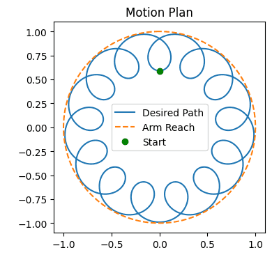
Ultimately we wanted to create a model of a robotic arm that would be able to follow an arbitrary motion path. In our example, we take a looping path and break it up into even time steps (but our method would work for any desired velocity/acceleration along the path).

We defined a circular/looping motion path and split it up evenly over an amount of time. Our goal was to move the end-effector to each point at the calculated time. Thus, we calculated the velocity needed between every two points over their difference in time.

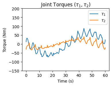
We inputted the desired locations, time, and velocities to reach each subsequent point into our inverse dynamics model, yielding us a torque value between each segment of points.

Inverse Dynamics Animation

As a bonus, we fed the torques back into the forward dynamics model to simulate the robot:

$$\begin{align*} \ddot{\theta} = M(\theta)^{-1}(\tau – C(\theta,\dot{\theta})\dot{\theta} – G(\theta)) \end{align*}$$

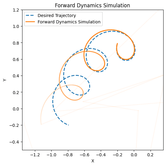
However, the system diverges very quickly and easily.

Limitations

Our forward dynamics simulation diverges due to a large number of reasons including: numerical approximations, estimations we made over the time step between points, starting velocity discrepancies, etc. In the real world, we introduce an error term in the inverse dynamics model to account for drag, friction of the motor, the motor’s dynamics changing due to heat/wear, the measurements not being precisely accurate, etc.

The next logical step would be to (in all modern control systems) is to incorporate proportional/integral/derivative controls to influence damping and rigidity of the motion and correct for small disturbances. All to say, we have only begun to explore the complexities of robotic control systems.

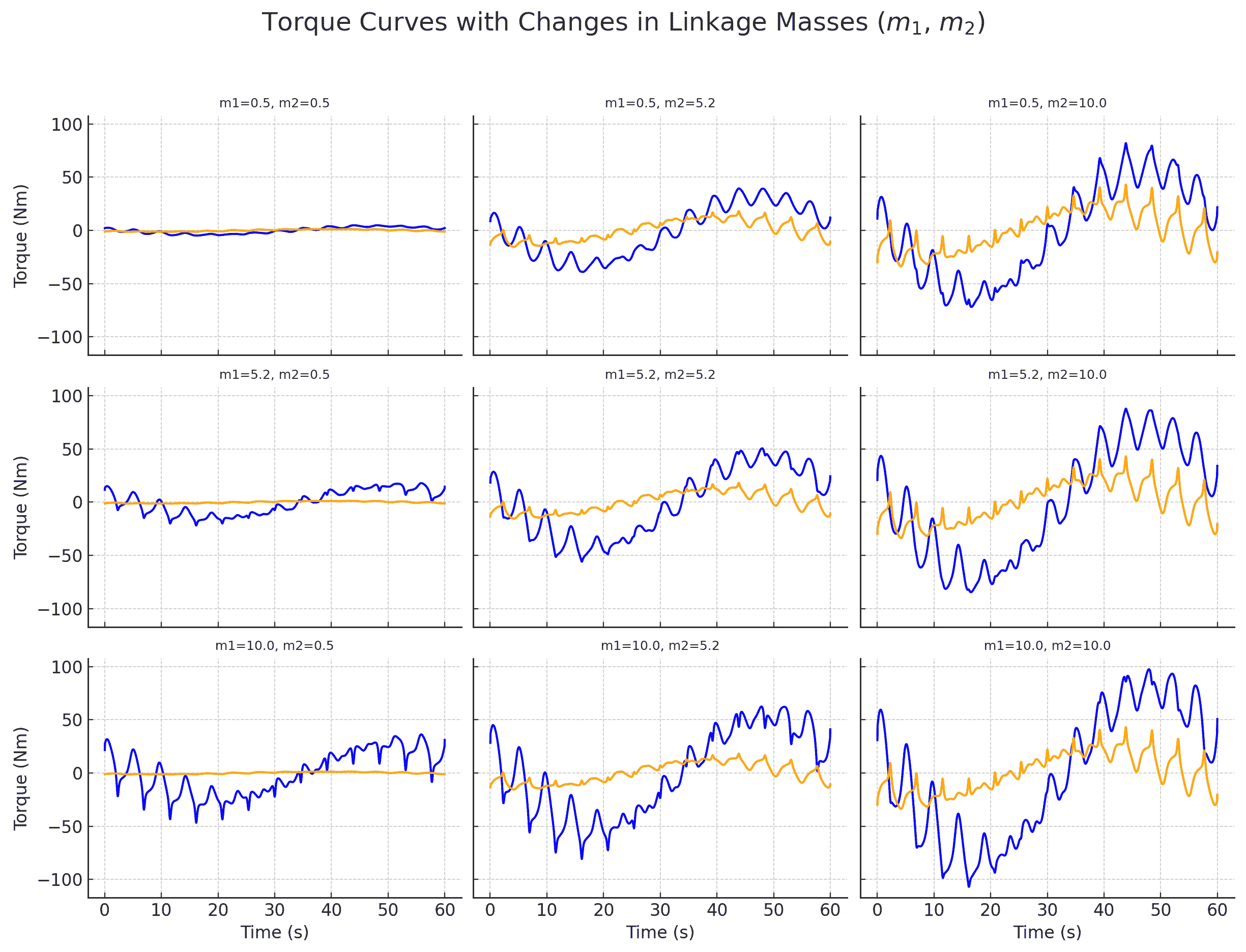
Parameter Sweep (Linkage Masses)

Code

We include only the code to calculate the inverse dynamics of the robotic arm as well as plot the desired path and output torques.

import numpy as np
import matplotlib.pyplot as plt
scale   = 0.79 # circle radius
radius  = 0.2  # loop radius
freq    = 13   # number of loops around circle
T_total = 60.0 # total motion time (s)
N       = 2000 # number of time steps / path points
t = np.linspace(0, T_total, N) # time vector
# create the looping path along the circle

# generate uniform circular base path
phi = np.linspace(0, 2*np.pi, N) + np.pi/2 # rotate so the starting point is at the top

path_base = scale * np.column_stack((np.cos(phi), np.sin(phi)))

# add loops, evenly sampled along the base path
def tangent_normal_frame(path):
    d = np.gradient(path, axis=0)
    lengths = np.linalg.norm(d, axis=1, keepdims=True)
    lengths[lengths == 0] = 1.0
    Tvec = d / lengths
    Nvec = np.column_stack((-Tvec[:,1], Tvec[:,0]))
    return Tvec, Nvec

def add_loops(path, radius, freq):
    N = len(path)
    u = np.linspace(0, 1, N)
    angles = 2 * np.pi * freq * u + np.pi/2 # fixes loop phase

    Tvec, Nvec = tangent_normal_frame(path)
    offsets = ( radius * np.cos(angles)[:,None] * Tvec + radius * np.sin(angles)[:,None] * Nvec )
    return path + offsets

loopy_path = add_loops(path_base, radius, freq)

def inverse_kinematics_both(x, y, l1, l2):
    r2 = x*x + y*y
    cos2 = np.clip((r2 - l1*l1 - l2*l2) / (2*l1*l2), -1, 1)
    th2_up = np.arccos(cos2)
    th2_down = -th2_up
    def th1(th2):
        k1 = l1 + l2*np.cos(th2)
        k2 = l2*np.sin(th2)
        return np.arctan2(y, x) - np.arctan2(k2, k1)
    return (th1(th2_up),   th2_up), (th1(th2_down), th2_down)

def compute_joint_trajectory_both(path, l1, l2):
    N = len(path)
    thetas = np.zeros((N,2))
    # seed with our preferred branch (elbow to the right)
    thetas[0] = inverse_kinematics_both(*path[0], l1, l2)[0]

    for i in range(1, N):
        sol_up, sol_down = inverse_kinematics_both(*path[i], l1, l2)
        # pick the one with smaller wrapped distance
        if dist_cfg(sol_up,   thetas[i-1]) <= dist_cfg(sol_down, thetas[i-1]):
            thetas[i] = sol_up
        else:
            thetas[i] = sol_down
    return thetas

# smallest signed difference between angles
def wrap_delta(a, b):
    d = a - b
    # wrap into [–\pi, +\pi)
    return (d + np.pi) % (2*np.pi) - np.pi

# euclidean distance in terms of joints (with wrapping)
def dist_cfg(cfg1, cfg2):
    d1 = wrap_delta(cfg1[0], cfg2[0])
    d2 = wrap_delta(cfg1[1], cfg2[1])
    return np.hypot(d1, d2)

def finite_diff_angles(arr, t):
    dt = t[1] - t[0]
    delta = wrap_delta(arr[1:], arr[:-1])
    diffs = delta / dt
    t_mid = (t[:-1] + t[1:]) / 2
    return t_mid, diffs

# robot configuration
params = {
    'l1':0.5, 'l2':0.5,
    'm1':1.0, 'm2':10.0, # top link heavier for greater effect on torque plots
    'I1':(1/12)*1.0**2,
    'I2':(1/12)*10.0**2,
    'g': 9.81
}

thetas = compute_joint_trajectory_both(loopy_path, params['l1'], params['l2'])
t_v, vel = finite_diff_angles(thetas, t)
t_a, accel = finite_diff_angles(vel, t_v)

torques = []
for (th1, th2), (d1, d2), (dd1, dd2), ti in zip(
        thetas[1:-1], vel, accel, t_a):
    M = M_matrix(th2,
                   params['l1'], params['l2'],
                   params['m1'], params['m2'],
                   params['I1'], params['I2'])
    C = C_matrix(th2, d1, d2,
                   params['l1'], params['l2'],
                   params['m2'])
    Gv = G_vector(th1, th2,
                   params['l1'], params['l2'],
                   params['m1'], params['m2'],
                   params['g'])
    tau = M.dot([dd1, dd2]) + C.dot([d1, d2]) + Gv
    torques.append((ti, tau[0], tau[1]))

times, tau1, tau2 = map(np.array, zip(*torques))

fig, (ax1, ax2) = plt.subplots(2, 1, figsize=(4, 7), gridspec_kw={'height_ratios': [3, 2]})

# top plot is the looping path and the circular reach of the arm
ax1.plot(loopy_path[:,0], loopy_path[:,1], label="Desired Path")
unit_circ = np.column_stack((np.cos(phi), np.sin(phi)))
ax1.plot(unit_circ[:,0], unit_circ[:,1], '--', label="Arm Reach")
ax1.plot(loopy_path[0,0],  loopy_path[0,1],  'go', label='Start')

ax1.set_aspect('equal', 'box')
ax1.set_title("Motion Plan")
ax1.legend()

# top plot is torques
ax2.plot(times, tau1, label=r"$\tau_1$")
ax2.plot(times, tau2, label=r"$\tau_2$")
ax2.set_xlabel("Time (s)")
ax2.set_ylabel("Torque (Nm)")
ax2.set_title(r"Joint Torques ($\tau_1, \tau_2$)")
ax2.set_ylim(-150, 200)
ax2.legend()

plt.tight_layout()
plt.show()

def M_matrix(th2, l1, l2, m1, m2, I1, I2):
    M11 = I1 + I2 + (m1*(l1*l1))/4 + m2*((l1*l1) + (l2*l2)/4 + l1*l2*np.cos(th2))
    M12 = I2 + (m2*(l2*l2))/4 + ((l1*l2)/2)*np.cos(th2))
    M22 = I2 + (m2*(l2*l2))/4
    return np.array([[M11, M12],
                     [M12, M22]])

def C_matrix(th2, th1_dot, th2_dot, l1, l2, m2):
    h = -m2 * l1 * (l2/2) * np.sin(th2)
    return np.array([[h*th2_dot, h*(th1_dot+th2_dot)],
                     [-h*th1_dot, 0.0]])

def G_vector(th1, th2, l1, l2, m1, m2, g=9.81):
    g1 = (((m1*l1)/2 + m2*l1)*g*np.cos(th1)
          + m2*(l2/2)*g*np.cos(th1+th2))
    g2 = m2*l2/2*g*np.cos(th1+th2)
    return np.array([g1, g2])

Note: the function for the Coriolis matrix is a slightly different variation from the one we derived since this one is more commonly used in computation by toolkits/libraries/etc.

Download the project PDF or the project \( \LaTeX \) project ZIP.

References

1. engrprogrammer. Two link robotic manipulator modelling and simulation on Matlab. Available at: https://youtube.com/shorts/RKZ0zjuxSvs?si=t6uC7lh3tqJkBYve
2. MATLAB & Simulink. LTV Model of Two-Link Robot. Available at: https://www.mathworks.com/help/control/ug/linear-time-varying-robot-model.html
3. MATLAB & Simulink. Derive and Apply Inverse Kinematics to Two-Link Robot Arm. Available at: https://www.mathworks.com/help/symbolic/derive-and-apply-inverse-kinematics-to-robot-arm.html
4. Northwestern Robotics. Modern Robotics, Chapter 8.1: Lagrangian Formulation of Dynamics. Available at: https://www.youtube.com/watch?v=1U6y_68CjeY
5. Northwestern Robotics. Modern Robotics, Chapter 11.2.1: Error Response. Available at: https://www.youtube.com/watch?v=ddkUszFVTUk&list=PLggLP4f-rq02N54sD6xwdDWlDScvb32Pp&index=2
6. Northwestern Robotics. Modern Robotics, Chapters 9.1 and 9.2: Point-to-Point Trajectories. Available at: https://www.youtube.com/watch?v=0ZqeBEa_MWo&list=PLggLP4f-rq00wo1z_Or2rRPAt1pStwmlY&index=2